Understanding Recurrent Neural Network and Long Short-Term Memory

Recurrent Neural Network (RNNs) are popular models that have shown great success in many NLP problems. But it seems that there is a limited number of resources that thoroughly explain how RNNs work, and how to implement them. Today, we are happy to share with you some basic knowledge about Recurrent Neural Network and a modified version of recurrent neural networks called Long Short-Term Memory which can resolved some problems of RNNs.

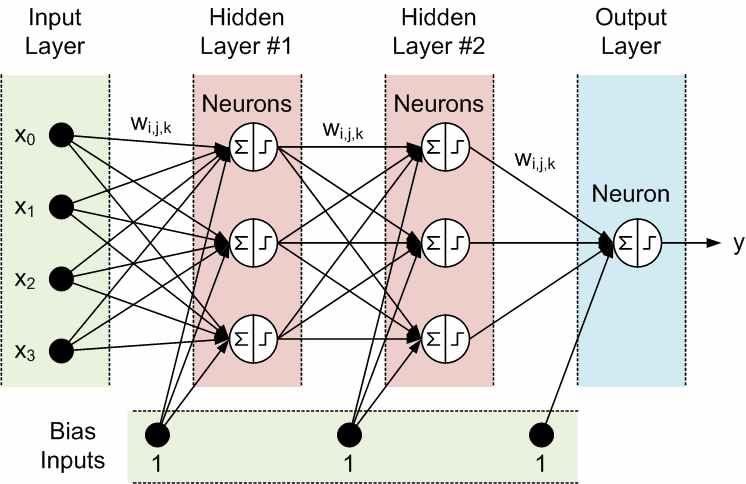
The Neural Network consists of 3 main parts are the Input layer, Hidden layer and Output layer. We can see that all inputs (and outputs) are independent of each other but for a large number of tasks, it’s a bad idea. Thus this model is not suitable for string problems such as description, sentence completion which are related to the next predictions. If you want to predict the next word in a sentence you better know which words came before it. RNNs are called recurrent because they perform the same task for every element of a sequence, with the output being dependent on the previous computations. Another way to think about RNNs is that they can be considered as a “memory” which captures information about what has been calculated so far. In theory, RNNs can make use of information in arbitrarily long sequences, but actually in practice, they are limited to looking back only a few steps. If you still do not understand anything, let’s take a look at the following RNN network model and analyze it to better understand:

In neural networks, a hidden layer is located between the input and output of the algorithm, in which the function applies weights to the inputs and directs them through an activation function as the output. In short, the hidden layers perform nonlinear transformations of the inputs entered into the network. Hidden layers vary depending on the function of the neural network, and similarly, the layers may vary depending on their associated weights.

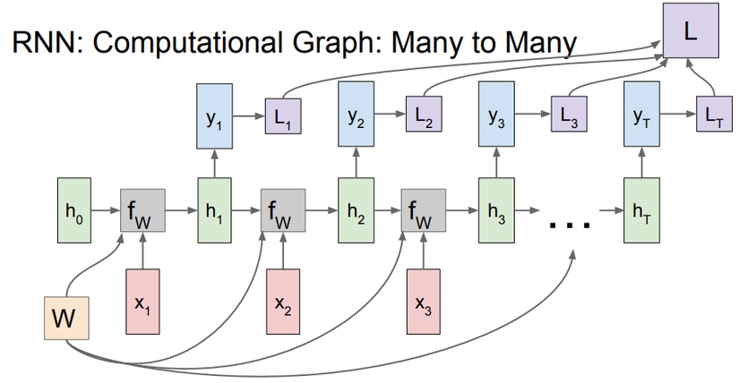
The input x(t) will be combined with the hidden layer h(t-1) by the function W(f) to calculate the current hidden layer h(t) and the output y(t) will be calculated from h(t). W is the set of weights and it is in all clusters, the L(1), L(2), .., L(t) are the loss functions that will be explained later. Thus the results from the pre-calculated processes were “remembered” by adding h(t-1) in order to calculate h(t). By doing this way, it allows increasing the accuracy of current predictions. To be more specific:

• x(t) is the input at time step. For example, could be a one-hot vector corresponding to the second word of a sentence.
• h(t) is the hidden state at time step. It’s the “memory” of the network. h(t) is calculated based on the previous hidden state and the input at the current step: h(t) = f(h(t-1), x(t)) The function usually is a nonlinearity such as tanh or ReLU. h(t-1), which is required to calculate the first hidden state, is typically initialized to all zeroes.
• y(t) is the output at step. For example, if we wanted to predict the next word in a sentence it would be a vector of probabilities across our vocabulary. 

There are a few things to note here:

•  The hidden state h(t) can be considered as the memory of the network. h(t) captures some information about what happened in all the previous time steps. The output at step y(t) is calculated only based on the memory at time. As briefly mentioned above, it’s a little bit more complicated in practice because h(t) typically can’t capture information from a huge number of time steps ago.
• Unlike a traditional deep neural network, which uses different parameters at each layer, a RNN shares the same parameters for all steps. It is the fact that we are performing the same task at each step, just with different inputs. This greatly reduces the total number of parameters that need to learn.
• The above diagram has outputs at each time step, but depending on the task this may not be necessary. For example, when predicting the sentiment of a sentence we may only care about the final output, not the sentiment after each word. Similarly, we may not need inputs at each time step. The main feature of RNNs is their hidden state, which captures some information about a sequence.

RNNs have seen great success in many NLP (Natural Language Processing) tasks. While LSTMs (Long Short-Term Memory) are a kind of RNN and function similarly to traditional RNNs, LSTMs are much better at capturing long-term dependencies than vanilla RNNs are. This feature addresses the “short-term memory” problem of RNNs. The key is that they just have a different way of computing the hidden state.

Long Short-Term Memory (LSTM) networks are the most commonly used type of recurrent neural networks, which makes it easier to remember past data in memory. The vanishing gradient problem of RNN is tackled here as LSTM is well-suited to classify, process, and predict time series given time lags of unknown duration. With LSTM, Deep Learning model will be trained by using back-propagation. In an LSTM network, three gates are present: Input Gate. Forget Gate and Output Gate.

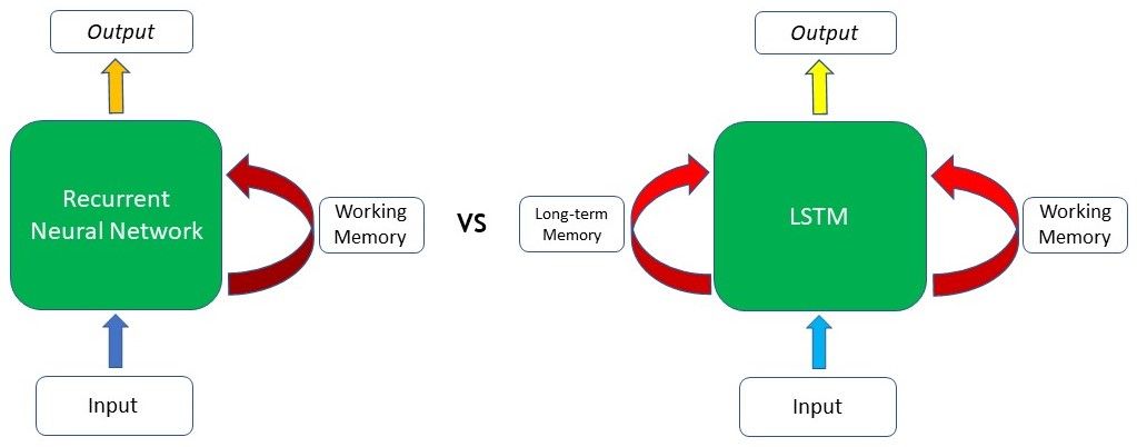
Looking at the image we can see that the difference lies mainly in the LSTM’s ability to preserve long-term memory which plays an important role in the majority of Natural Language Processing (NLP) or time-series and sequential tasks. For example, let’s imagine we have a network generating text based on some input given to us. At the start of the text, it is referred to the author having a “dog named Cliff”. After a few other sentences where there is no mention of a pet or dog, the author brings up his pet again, and it’s time the model needs to generate the next word to “However, Cliff, my pet ____”. As the word pet appeared right before the blank, a RNN will deduce that the next word will likely be an animal that can be kept as a pet.

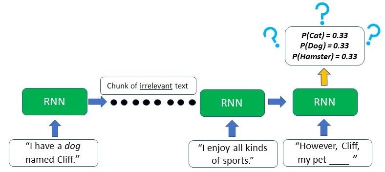
However, due to the short-term memory, the traditional RNN will only be able to use the contextual information from the text that appeared in the last few sentences – which is not useful at all. The RNN has no clue as to what animal the pet may be as the relevant information from the start of the text has already been lost. RNNs are unable to remember information from much earlier

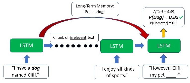
In contrast, the LSTM can retain the earlier information that the author has a pet dog, and this will assist the model in choosing “the dog” when it comes to generating the text at that point due to the contextual information from a much earlier time step.

LSTMs are explicitly designed to avoid the long-term dependency problem. Remembering information for long periods of time is practically their default behavior, not something they struggle to learn!

To help users to develop RNN models faster and more accurately, iRender has launched GPU Cloud for AI/DL service which is a computer rental service with powerful GPU and CPU configuration. We offer 6/12 cards x GTX 1080 Ti and 6/12 cards x RTX 2080 Ti, speeding up Training set, Cross-validation set, and Test set. If any help, contact us via email, our 24/7 technical support is always available – just a click iRender makes every effort to support our customers, thanks to our experts, software development teams, and technical directors available 24 hours, 7 days a week, even during major holidays.

Sign up here and use our services!

Nguồn: AI Global