Optimize Render Settings for Octane
Optimizing a render is a two-part process. In the previous article, we have learned how to optimize a scene in Octane. Once a scene is well-optimized, we will focus our efforts on the render settings for Octane. Let’s see what we need to do in this process with iRender.
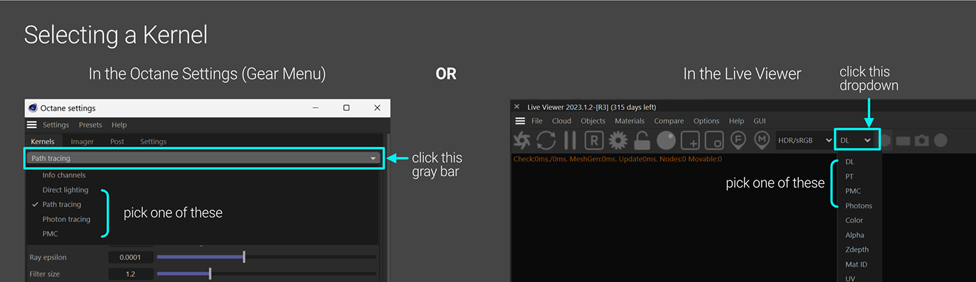
Step 1: Pick a kernel
The Kernel is the main chunk of code that Octane Render uses to render a scene. You can select it in the Octane Settings or the Live Viewer.
Currently, there are four kernel types which are Direct Light, Path Tracing, PMC, and Photon Tracing. As a general rule, the default kernel settings work well as a baseline. However, changing them based on the specific lights, materials and effects used in a scene can help optimize rendering.
Which kernel should we pick?
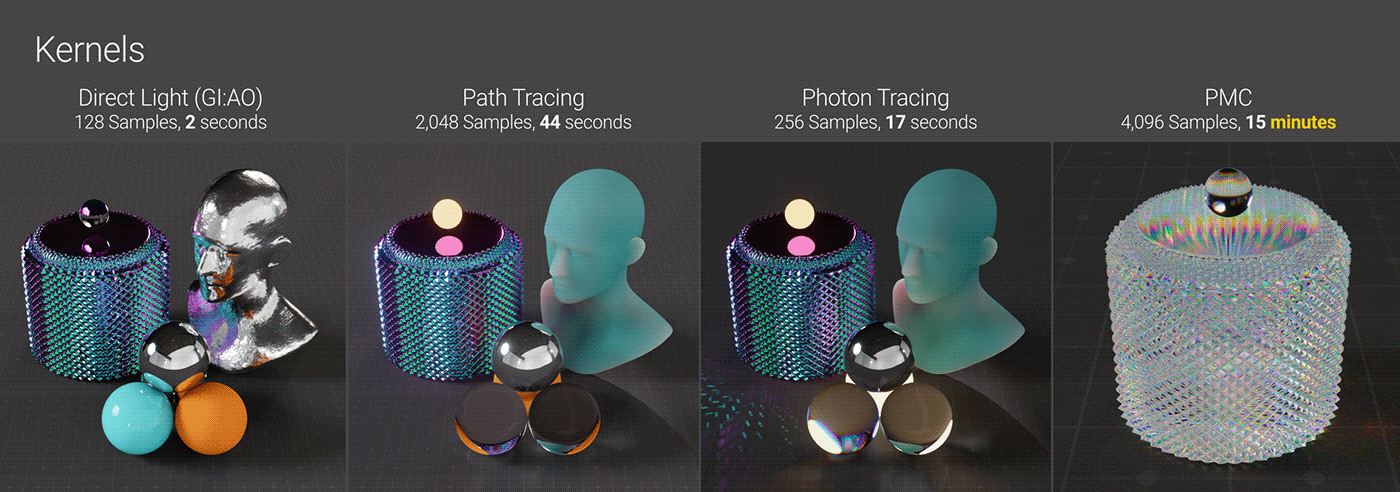
Direct Light (DL)
The Direct Light (DL) kernel is the most basic but still useful in some scenes and situations. It provides three Global Illumination modes that balance realism versus render speed. However, DL cannot produce caustics and has very limited scattering effects. So for scenes involving caustics or substantial scattering, the Path Tracing kernel would be preferable.
Path Tracing (PT)
The Path Tracing (PT) kernel builds upon Direct Light by providing improved calculations for secondary bounces, including caustics. It also enhances several settings to produce even more realistic results than DL can achieve. However, because PT relies on older techniques for secondary bounce, it can struggle to generate tight caustic patterns. It is also very prone to noise and fireflies if the settings are not carefully set. Despite these limitations, PT remains a suitable choice for scenes where caustics play a less central role.
Photon Tracing
The Photon Tracing kernel builds upon Path Tracing by adding a faster, more efficient and visually improved method for calculating caustics. It makes getting well-defined caustic patterns quick and easy while retaining all the realistic rendering advantages of Path Tracing. Photon Tracing is the solution where caustics play an important role in a scene but are not resolving well with Path Tracing.
One caveat is that it creates some computational overhead which could cause issues for multi-GPU or network rendering setups. Therefore, Photon Tracing is best considered only when truly needed, such as for scenes with complex lighting where caustics are important or causing problems that cannot be handled through other Path Tracing tweaks.
PMC
PMC is somewhat distinct from the other kernels. While it can produce caustics better than PT, it is significantly slower and incompatible with Octane’s pre-2024 denoiser and adaptive sampling. Using a different ray calculating algorithm, PMC results in a unique look. It may be preferable only in scenes with extremely complex lighting and refraction, though at the cost of much longer render time. PMC is also less predictable between frames than PT or Photon Tracing, making it not great for animation.
When considering PMC, you should initially lookdev at PT or Photon Tracing, then test PMC in the process once the scene is mostly complete to see if it better handles extreme complexity.
Step 2: Set initial settings
When setting up the initial settings for any kernel, a good strategy is to set sample counts low but increase all other settings. This minimizes the risk of missing important calculations that occur with overly restricted bounces or clamping, while also reducing unnecessary processing from high samples at the initial setup stage. The optimization process then involves gradually lowering other values and slowly raising the maximum samples until reaching a balanced configuration.
-
- Turn on AI Light if we are using physical lights.
- Turn off Denoiser while doing the initial lookdev, only turn it on at the end of the process when we are happy with the overall look.
- Start Parallel samples at 32 (lower if having less VRAM).
- Choose the tone mapping now (using ACES or AgX tone mapping will create a very different visual appearance compared to no tone mapping in sRGB).
For Direct Light: 16-64 maximum samples should be sufficient. When using the GI_Diffuse mode, increasing the diffuse bounce to 5 is recommended. This setting is ignored for the other GI modes. If the scene contains glass or lots of metal materials, increasing the Glossy and Specular bounces to 8 is a good idea to improve reflection/refraction calculations. Otherwise, the default settings for other bounce parameters are good.
For Path Tracing and Photon Tracing: set the maximum samples between 64-256 depending on GPU capability and complexity of scene elements. The default settings of 16 bounces for Diffuse and Specular, and a GI Clamp of 1,000,000 is a good starting point. Render quality may range from noisy to clean depending on the scene. Ensure the “allow caustics” option is enabled in the IOR channels of reflective and refractive materials that will produce caustics when using Photon Tracing.
For PMC: set the maximum samples between 256-1024. Since PMC takes longer to resolve details in caustics, it needs more samples even during lookdev.
Step 3: Cap the bounces
Depths
Depth, referred to in CG as “bounces” or “trace depth”, is the number of times direct rays bounce off or through an object. Optimizing bounce settings is one of the most effective ways to improve render speeds without raising noise or other artifacts. However, it needs to be done thoughtfully. Depth settings directly impact rendered scene information that cannot be cheated with post-effects. We should begin with higher bounce values to fully understand the scene’s intended look, then progressively reduce bounces to boost speed until reaching the point where quality and realism noticeably degrade.
All four Octane kernels have three different Depth settings. Direct Light has sliders for Diffuse, Specular, and Glossy. Path Tracing, Photon Tracing, and PMC have sliders for Diffuse, Specular, and Scatter.
Glossy Depth
Glossy Depth is only in the Direct Light (DL) kernel. It affects bounces off of reflective materials having Specular or Metallic contributions, and it does not affect transmissive (glass/liquids/etc) materials.
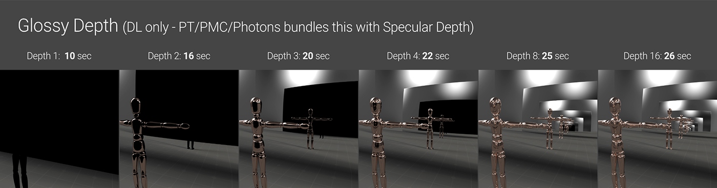
A helpful way to understand this effect is using a “hall of mirrors” test scene as shown above. With insufficient bounces, anything that would reflect additional times will be rendered as black. At a minimum, two bounces are needed to display any reflective surfaces. Lower values quickly black out sections, while higher values reduce black patches to an unnoticeable size, similar to reality. 16 bounces typically work well unless a scene is entirely made up of mutually reflective objects.
The Direct Light kernel defaults to just 2 bounces, likely too low for scenes with metals or glossy materials. Bump this up initially to 5 or 8 bounces minimum, then gradually reduce it to optimize quality versus performance as reflections blackening is observed.
Specular Depth
Specular Depth is in all kernels. In Direct Light, it only affects transmissive materials (glass, liquids, etc), while it affects both reflective (glossy/metallic) and transmissive materials in the other 3 kernels.
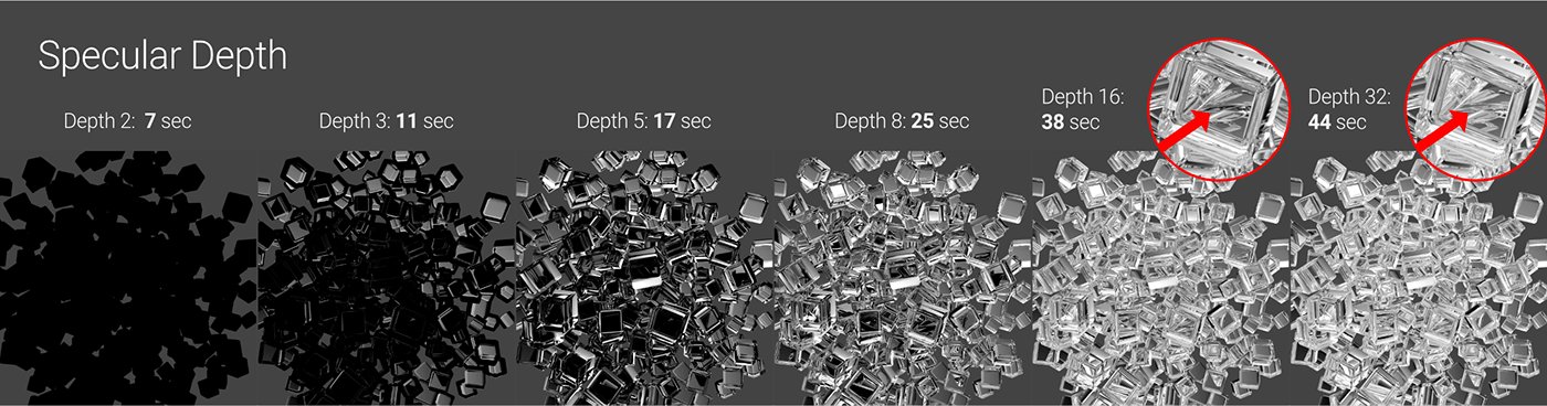
A minimum of 3 bounces is needed to see anything through a transmissive material, which may suffice for simple scenes but is likely insufficient for more complex scenes. 5 bounces is a reasonable starting point, or 8 if we have lots of refraction.
The default of 16 bounces for PT, PMC and Photon Tracing kernels usually works well as it also impacts reflections. Scenes with overlapping glass and metals could potentially require 32 bounces to fully resolve tricky refracted areas. Heavy refraction places high demands on the GPU and render times, so optimizing this setting through testing is important.
Diffuse Depth
Diffuse Depth setting is found in all four rendering kernels. It determines the number of bounces rays can undergo off of materials containing a diffuse/albedo/base color component. Diffuse Depth is a little more complex than glossy or specular bounce settings as it more heavily influences indirect or secondary ray bounces rather than direct rays.
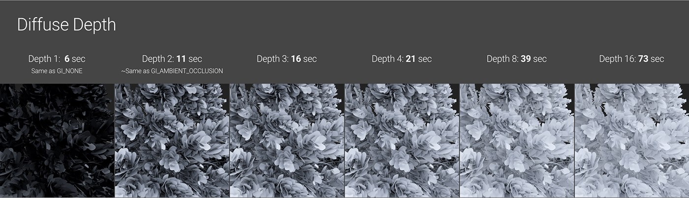
Unlike reflections or refractions, insufficient diffuse depth will not result in areas being fully blacked out, as diffuse materials do not exhibit hard cutoffs in the same way. Instead, the main observable effect of increasing the diffuse depth slider is a gradual brightening and softening of diffuse geometry as more light bounces off those surfaces. The degree of brightness change depends heavily on the material’s diffuse/albedo color – darker tones absorb more light with each bounce.
Scatter Depth
Scatter Depth is available within the PT, PMC and Photon Tracing kernels. Some types of scattering effects involving diffuse transmission can also be achieved using the Direct Lighting kernel, but only when it is in GI_DIFFUSE mode, with the scene look then controlled via Diffuse Depth. Even so, because the Direct Lighting kernel does not have a Scatter Depth parameter, it’s better to use other kernels for sub-surface scattering, fog or other transmissive scattering effects.
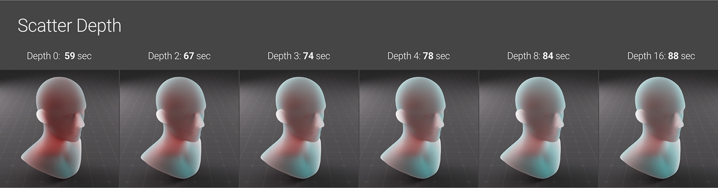
Scatter Depth determines the number of internal bounces in a scattering media such as sub-surface scattering or volumetric fog. However, it is only one part of the equation – achieving the desired look requires carefully balancing Scatter Depth with other factors like Max Samples, Medium Density, Volume Step Length, scene lighting, and three or four other things.
The visual impact of increasing Scatter Depth can vary significantly based on the interplay of related settings. In the below example, the difference between 0, 2 and 3 bounces is noticeable, but 3 to 16 bounces yield a minor, despite adding 14 seconds to the render time per frame.
GI Clamp
Path Tracing, Photon Tracing, and PMC simulate indirect lighting more realistically than Direct Light. They account for caustics, which occur when light bounces off a reflective surface or through a refractive one before settling on a diffuse surface. Calculating caustics and secondary bounces places high demands on the GPU but greatly increases realism. In reality, infinite indirect light bounces illuminate the environment, but render engines have limited resources. If the simulation is not given sufficient time to resolve properly, artifacts emerge as noise and hot pixels (sometimes called fireflies).
GI clamp is a tool that helps mitigate these artifacts. It compresses the contribution of indirect rays. It acts as a filter, limiting strong, independent indirect rays that could otherwise generate isolated hot pixels early in the progressive sampling process. By limiting the rays, the GI clamp trades off some realism in the scene but helps eliminate noise and hot pixels from caustics caused by Path Tracing and PMC kernels.
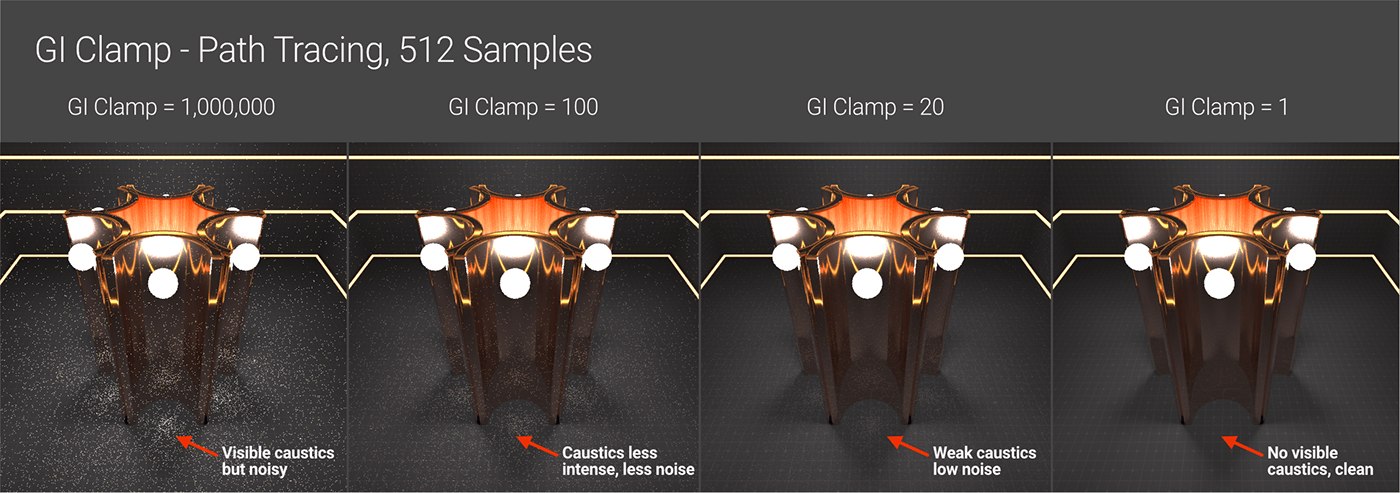
The default GI Clamp value of 1,000,000 essentially imposes no limitation. Setting the GI clamp to 1 results in an image appearance very similar to, and sometimes exactly matching, Direct Lighting using GI_Diffuse mode. For scenes without significant interior lighting or caustics, very low GI clamp values such as 100 or even 10 can suffice.
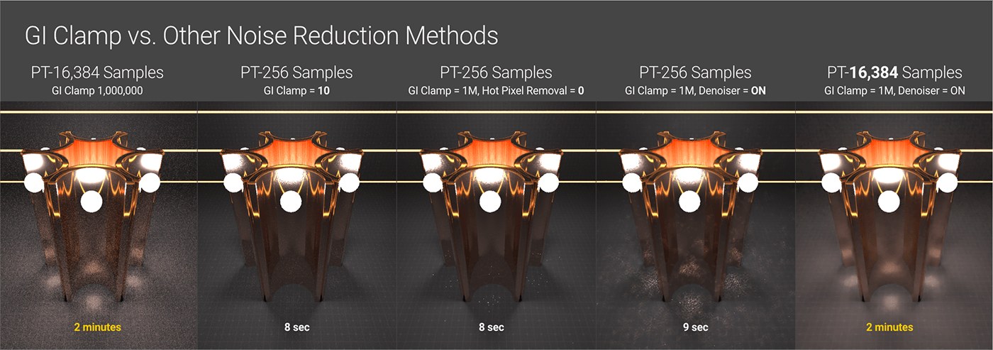
Increasing Max Samples alone may reduce noise through brute force computation, but usually not enough to fully eliminate it. The Denoiser and Hot pixel removal tools can help. However, relying too heavily on these tools risks introducing other artifacts such as blurry/splotchy areas or unwanted alterations, especially for animations. Ideally, the GI clamp value should remain as high as possible. If the noise and hot pixels are caused by caustics, we then should switch to the Photon Tracing engine to resolve most of that. If the lights are problems, we can use the techniques to solve them. After using these techniques, we then lower the GI clamp value to clean up any stubborn noisy areas.
Step 4: Optimize the Calculations
AI light
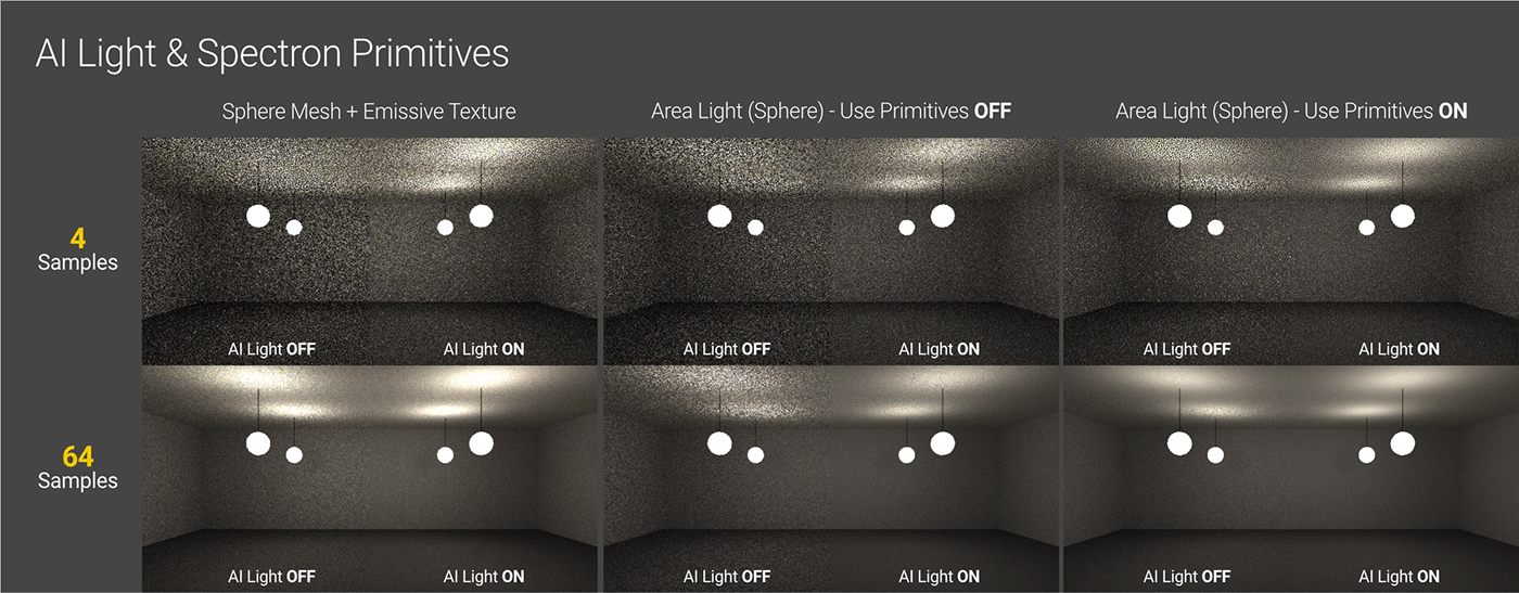
For scenes with many area lights, using AI/Analytic lights can speed up the lighting calculations. In simpler scenes, these light types may not provide benefits and could potentially increase processing overhead instead.
Parallel Samples
This is hardware and scene-dependent and has to do with optimizing the number of GPU cores being used at one time. Higher values can increase render speeds by better-utilizing cores, but use more VRAM. As a starting point, a value of 32 is suitable for modern cards on average scenes, while 16 works better for older cards with less VRAM and/or heavy memory scenes.
Step 5: Dial in Sampling
After resolving as much of the noise and problem areas but still maintaining the look we want, we can go back to the overall sampling of the scene to determine the final quality. Each scene is different, so there is no rule here.
Render Settings for Octane: Max Samples
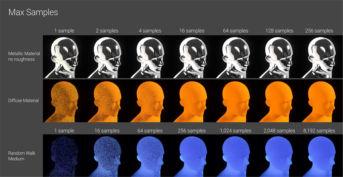
The four Octane kernels use progressive passes, referred to as samples. When rendering begins, Octane sends out rays to generate a low-quality initial image using quick calculations based on lights, geometry and materials. This is the first sample, the first pass. It then does the same thing again and returns another slightly better version – the second sample. It continues to refine until it hits the maximum sample number set in the Max Samples field.
Direct Lighting typically requires far fewer samples than other kernels as it cannot produce advanced effects like caustics. This explains why its default of 128 samples in C4D.
The other three kernels must account for effects like caustics and secondary bounces, which are complex to simulate. Since Octane cannot know precisely what each scene entails, its default max sample count is set relatively high at 16,000 samples when used in C4D. This number is usually enough to eventually resolve most scenes, regardless of optimization in other settings.
However, rendering at 16,000 samples takes a long time and is unnecessary for simpler scenes that converge more quickly. The goal across kernels and scene complexity is to find the minimum samples needed for acceptable quality, not perfectly optimized. Precisely testing small sample increments is inefficient, as render time would be better spent optimizing other factors or other priorities. The approach aims to approximate, not exactly determine, the lowest sample count that balances image quality versus efficiency through testing.
Adaptive Sampling
While max samples are like a brute-force way of reducing noise, adaptive sampling offers a more optimized method. Adaptive sampling optimizes this process by stopping sampling in image areas that it determines are already well-resolved, then increasing the sampling more heavily in still noisy areas. By concentrating effort only on the areas requiring it, adaptive sampling can significantly speed up the rendering process.
Note: DL, PT, and Photon Tracing support Adaptive Sampling, but PMC does not.
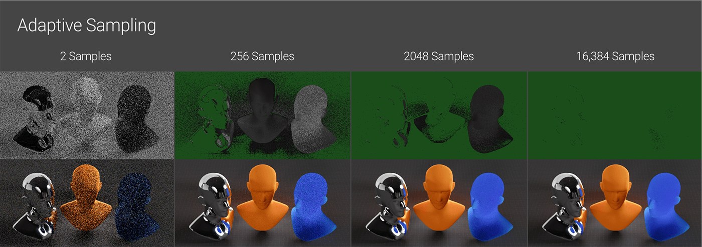
Scenes that contain lots of noise in particular areas may experience a notably faster overall render time. Scenes with a uniformly distributed level of difficulty across the frame are unlikely to be affected.
The scene shown above would be well-suited for adaptive sampling. The top row shows how noise is reduced over time – sections turning green have been fully resolved and do not receive further processing. The metal on the left took no time to render, the diffuse material in the middle required around 1,000 samples, and the subsurface scattering on the right was extremely challenging for the GPU needed the full 16,000 samples to clean up.
It took 16,384 samples to fully resolve the whole scene with and without Adaptive Sampling. However, it took specifically 1:07 to fully render the scene with adaptive sampling on, compared to 3:30 to render without it. This is because, towards the end, Octane only had to worry about the SSS head, so it could burn through those remaining samples much faster.
AI Denoiser
Once the other details have been settled, we can examine if denoising can help speed up render times. Denoising is a post-processing effect in Octane Settings’s Imager tab that waits until the rendering is complete. It then applies a magical algorithm to analyze different image areas and remove what it considers noise. Using Denoiser allows us to stop the rendering process earlier than usual and still achieve a final product. So, let’s set up Denoiser in the render setting for Octane.
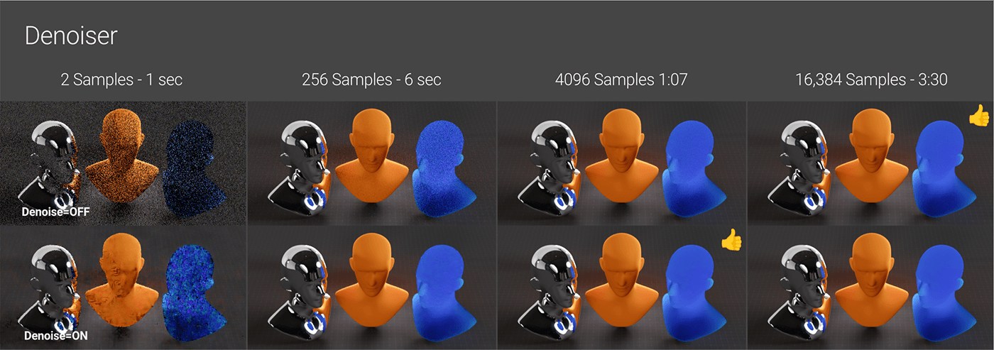
In the example above, the denoiser did an excellent job on the metal area even at just 2 samples, since it was mostly resolved already. It performed poorly on the diffuse material and very poorly on the subsurface scattering, as it did not have much data to work with. By 256 samples (in 6 seconds), the metal and diffuse areas were almost complete, and the SSS was improving. We could potentially stop the render somewhere between 3072 (in 50 seconds) and 4096 (in 1m07s) samples and consider the denoised result the final image. Without denoising, the SSS still had noticeable noise after 16k samples and over 2+ minutes of rendering.
Sometimes with denoising, areas of large, smooth organic surfaces may only require a fraction of the samples to get clean. In other cases, intricate patterns may get lost or look blurry because the denoiser incorrectly identified them as noise, and only a few seconds are saved by the time enough samples produce an acceptable appearance. The effectiveness of the Denoiser depends entirely on the scene being rendered.
A sound method is to render the image as clean as possible without using a denoiser. Then, apply the denoiser and gradually decrease the maximum sample count to find the lowest number that still maintains rendering quality. This may reduce minimum samples and noise threshold if combined with adaptive sampling.
Note: Denoising can introduce undesirable effects like jitter or moving artifacts in animation if relied on too heavily. To avoid wasting time, it is best to first render a subset of frames or a specific region for an animation to ensure the whole frames would not end up being unusable.
Tone Mapping
Tone Mapping does not directly optimize the rendering process, but it still affects how lights and materials are set up.
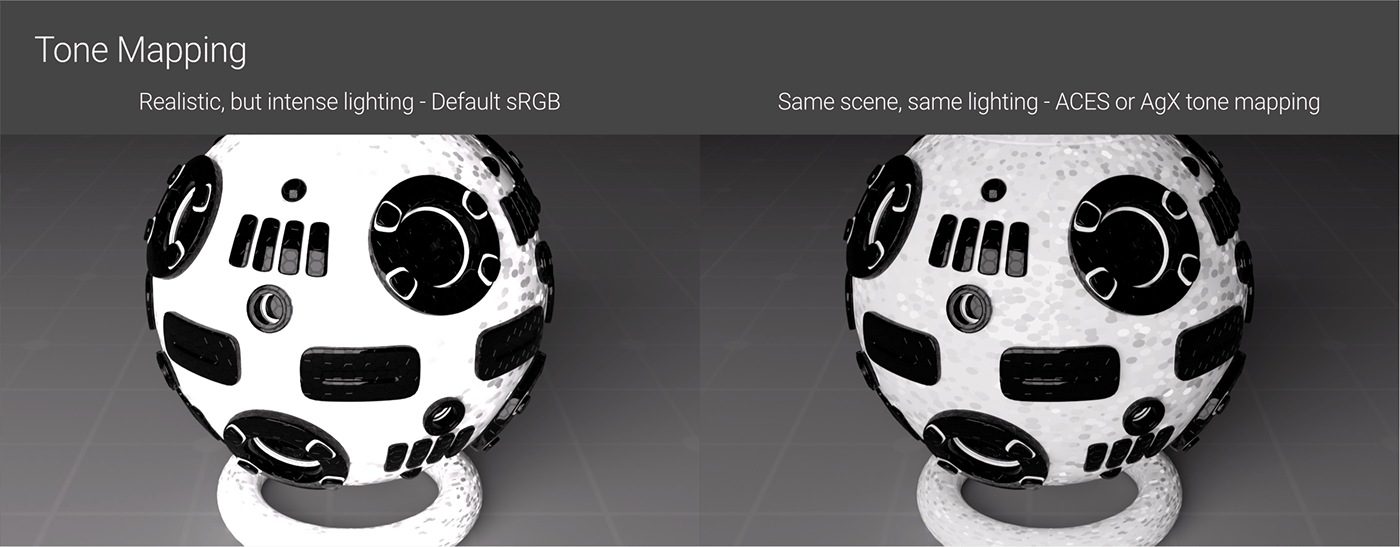
Using the default un-tone-mapped method could potentially lead to certain design decisions that then cause issues in other areas of the rendering.
Except for a few very specific cases like needing to match an exact sRGB hex value or going for a purposely non-photorealistic style, the default tone mapping method of simply clipping out-of-gamut values is never as good as an alternative such as ACES or AgX. Fortunately, Octane offers a one-click solution to use ACES tone mapping, and while setting up OCIO to work with AgX requires some initial configuration, it is straightforward to implement across all projects going forward.
In conclusion, optimizing a render in Octane requires attention to both the scene setup and render settings for Octane. Proper scene preparation with optimized textures, geometry and lighting avoids stressing the GPU. Once the scene is optimized, we shift to the render settings to pick up a kernel, limit rays, use some helper tools, decide the needed pass number, and even cheat a little with post to speed up rendering the final frames as fast as possible.
![]() iRender provides powerful render machines supporting all Octane (and its plugins) versions. Our GPU render farm houses the most robust machines from 1 to 8 RTX 4090/RTX 3090, AMD Threadripper Pro CPUs, 256GB RAM and 2TB SSD storage to boost rendering Octane projects of any scale. Check out our Octane GPU Cloud Rendering service to have more references and find the best plan for your Octane projects.
iRender provides powerful render machines supporting all Octane (and its plugins) versions. Our GPU render farm houses the most robust machines from 1 to 8 RTX 4090/RTX 3090, AMD Threadripper Pro CPUs, 256GB RAM and 2TB SSD storage to boost rendering Octane projects of any scale. Check out our Octane GPU Cloud Rendering service to have more references and find the best plan for your Octane projects.
Reference source: Scott Benson
Related Posts
The latest creative news from Octane Cloud Rendering.