10 tricks for better Houdini FLIP fluid simulations

Houdini provides a powerful set of tools when it comes to simulating fluids. However, it’s always a challenge to make fluids look realistic, especially for broadcast work.
In this article, let’s explore some hacks from FuseFX artist Kevin Pinga, to create faster, more flexible Houdini FLIP fluid simulations.
1. Source fluids with POP Source, not FLIP Source
The one and default method to source fluid for Houdini FLIP is to use a FLIP Source node. It will create a VDB which is read in by the Volume Source node in DOPs. This way works fine when you’re sourcing from a large ambiguous shape; however, it can get quite resource-heavy and time-consuming before you even get to the simulation phase.
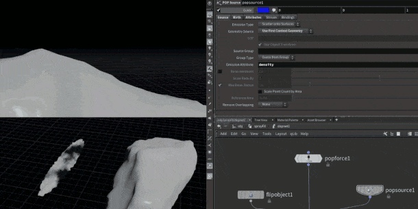
Instead, you should use regular polygon-based SOP geometry directly with no conversion to VDBs. This source can be read in by the POP Source node wired into the Sourcing input of the FLIP solver itself, in the same way that you would import a source for a regular particle simulation.
This method is more intuitive as you have been familiar with controls on the POP Source node through your time working with regular particles. You can control and monitor particles easily and independently of the Particle Separation of the FLIP object itself.
2. Use POP nodes with FLIP fluids
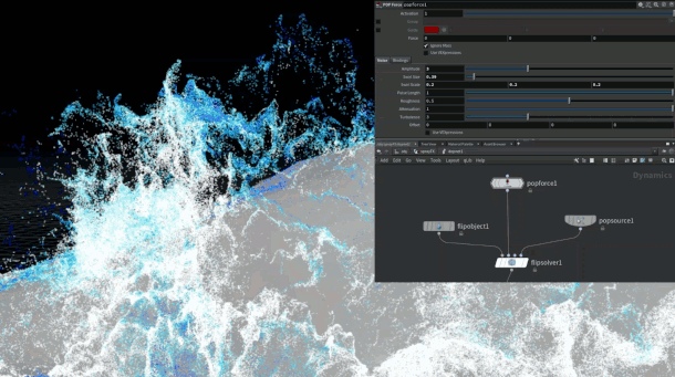
FLIP is essentially a series of POPs with some volumetric advection steps in between. However, the base itself is just particles, which means that all the POP nodes in DOPs can be used for FLIP fluids. This is why we were able to source using the POP Source node in the previous tip.
The POP Force node is a staple for creating interesting motion when working with regular particles. So we can use it with FLIP fluids too. Using it to introduce even a small amount of noise can create a more appealing-looking fluid. Low-frequency noises can also be useful for creating detail without having to increase your particle count or particle separation. (Be careful not to add too much noise, as this can cause unrealistic simulation.)
Another POP node that is useful in FLIP simulations is POP Speed Limit. Coupled with a POP Drag node, it works great for controlling high-velocity particles that can otherwise go out control.
3. Use Bounds qL to set your FLIP limits
The Bounds qL node is a very useful tool that packs in many simple features. It comes as part of a larger open-source Houdini toolset called qLib. In most studios, qLib is installed by default. If it’s not in your personal production environment, you can install yourself by following the instructions on GitHub.
Kevin Pinga shares that he uses Bounds qL primarily for setting his volume limits for FLIP and Pyro simulations. This is a step up from the standard Bound node as it includes an option to create bounds based on an animated input.
The most useful feature is the Output: Values checkbox, which unlocks the values of the size and center of the bounding box. These values can then be copied to any parameter in the FLIP solvers’s Volume Limits tab, or any other operations that require a bounding box. Having centralised bounding box info can avoid user error and helps in creating more procedural setups.
4. Enable useful attributes in the FLIP solver
There are three main parameters on the Houdini FLIP solver which you should turn on in your FLIP sims: ID, age and vorticity. They can be used to make post-simulation tweaks, and can all be found in the FLIP Solver under the Behavior and Vorticity tabs.
Most artists are already familiar with the ID attribute and how powerful it can be. Your data size might take a small hit for caching an additional attribute, but it’s always a good idea to have that information available.
You can control how a sim looks over time by enabling the age attribute via the Age Particles checkbox (which also exports the life attribute). This is useful especially if you have a source that is constantly emitting.
The vorticity attribute is handy for sourcing secondary simulations like whitewater and is great for manipulating shading.
5. Do post-simulation tweaks to salvage failing sims
There is a tendency to rely heavily on the output of a Houdini FLIP simulation as a final result. While this is an ideal workflow, due to time constraints, you don’t always have the luxury of resimulating to fix problems. In cases like these, running post-simulation tweaks on the FLIP particles themselves can help ‘salvage’ the sim.
You also should add the ID attribute so that you can use the Retime node to retime a sim.
Pinga says that he encounters another common problem when running mid-res simulations. That is, the size of the liquid droplets is good in high-density areas of the simulation, but too big in sparser areas. In cases like this, a simple wrangle using the pcfind: function can help mark sparse areas and lower their pscale value.
Below is the code snippet used in the wrangle:
int pc[] = pcfind(0,’P’,@P,chf(‘max_dist’),chi(‘max_pts’));
@pscale *= float(len(pc))/ch(‘max_pts’);
6. Use xyzdist to handle high-resolution collision surfaces
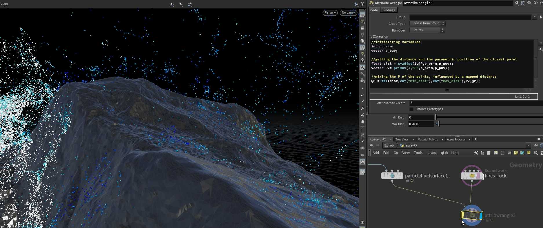
This is another post-simulation tweak. Together with primuv(), xyzdist() is by far the most useful.
In a VEX or VOPs context, xyzdist() calculates the distance to the closest interpolated point on a surface. When combined with primuv(), you can extract any attribute from the parametric UVs of the object!
In the case of the example above, we extract the position of the high-resolution collision surface and use it to push particles towards the surface. In some cases, you can also run this directly on the meshed surface itself, especially in shots where the collision surface is see-through (for example, pouring liquid into a clear glass). Clamping the distance to a really small value will help you to speed up calculations.
Here’s the code snippet used in the wrangle:
//initializing variables
int p_prim;
vector p_puv;
//getting the distance and the parametric position of the closest point
float dist = xyzdist(1,@P,p_prim,p_puv);
vector P2= primuv(1,”P”,p_prim,p_puv);
//mixing the P of the points, influenced by a mapped distance
@P = fit(dist,chf(“min_dist”),chf(“max_dist”),P2,@P);
In production, there is a more practical usage. You use a lower-resolution collider during simulation, and then run this function in a post-simulation wrangle to make the fluid look like it’s interacting with a high-res collider.
7. Kill problematic particles with ID
This is a simple yet effective trick when you have a simulation that is 98% close to being final, but where the remaining 2% of particles are just not working. If you stored the ID attribute mentioned in the previous tips, you can use it to blast away the problem particles. Without ID, you wouldn’t be able to mark the correct particles for deletion as the point count changes from frame to frame.
You can troubleshoot this by going into point selection mode and hit [9] on your numpad. This brings up the Group Selection pane. To select by ID, click on the gear icon and select Attributes > id. Now you can simply select the particles you want to remove in the viewport and hit [Delete]. A Blast node will be generated automatically referencing the point ID instead of the point number.
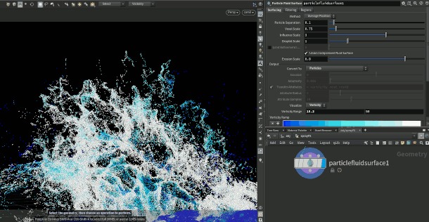
8. Use reseeding to beef up sparse regions

In production, sometimes you will meet a problem, in which the final render does not look correct as it doesn’t have enough particles. This is due to using a mid-resolution FLIP sim.
In cases like this, you should turn up the reseeding parameters instead of changing your particle separation. By default, reseeding is already turned on, but cranking up the Surface Oversampling parameter can help increase particle count in sparse areas by spreading out the particles. This way, you get to keep the general look of your simulation but have enough particles to avoid the meshed fluid looking incorrect.
9. Use the original Houdini FLIP sim directly as a different element

The traditional way to create whitewater is to simulate the FLIP fluid, then run the Whitewater solver on top of that. However, the second step isn’t always necessary, particularly for fast-moving fluids like splashes and water jets (think a broken fire hydrant or underwater in a hot tub). In addition, it can be quite tricky to get the fluid to look right when meshing the particles.
However, you can take the FLIP sim itself and render it directly with a whitewater shader. You can either render the particles themselves, or rasterize them to a VDB and render the result as a volume.
10. Optimise the sim and caches
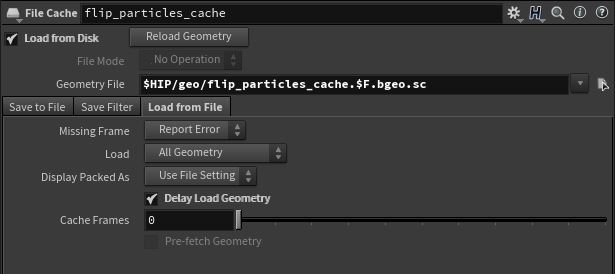
One of the challenges with high-resolution FLIP sims is dealing with the large amounts of data they generate. A common practice is to delete all the attributes that you don’t need before caching any part of a simulation.
Another thing that you can do to help reduce your memory footprint is to cull the particles outside the camera’s frustum. Additionally, if you have geometry that is ready to be rendered, it is a good idea to cache it out and have the Delay Load Geometry checkbox turned on. Instead of having Mantra embed the geometry in the IFD file, it will be referenced to the file on disk instead. This will help reduce load times and also drastically reduce both IFD generation times and file size.
Conclusion
Above are some hacks from Kevin Pinga when it comes to simulating fluids with Houdini FLIP solver. These tips and tricks can help you manage your fluid simulations more efficiently when trying to deliver fluid shots in a timely manner, while still maintaining a high level of quality.
iRender is proud to be one of very few render farms support Houdini rendering with powerful RTX3090. From single RTX3090, to dual 3090s and even 4x, 6x, 8x RTX3090s, we always have enough machine and config to serve your project.
Just 6 simple steps then you can connect to our powerful machine, install your Houdini and render engines (like Redshift, Octane, V-Ray, or Arnold, etc.), add your license then render/ revise your project as you want.
Not only those powerful configuration, iRender also provides you more services. From NVLink for large scene, to useful and free transferring tool named GPUhub sync. Our price is flexible with hourly rental which has pay-as-you-go basis, daily/ weekly/ monthly subscription with discount from 10-20%. Plus, you have 24/7 support service with real human who will support you whenever you encounter an issue.
Let’s see some of our Houdini with Redshift, V-Ray, Arnold and Octane benchmark:


Register an account today to experience our service. Or contact us via WhatsApp: (+84) 916806116 for advice and support.
Thank you & Happy Rendering!
Source: cgchannel.com
*Note: All images in this article are from cgchannel.com
Related Posts
The latest creative news from Redshift Cloud Rendering, Houdini Cloud Rendering , Octane Cloud Rendering, 3D VFX Plugins & Cloud Rendering.